User Guide
Layout of the interface
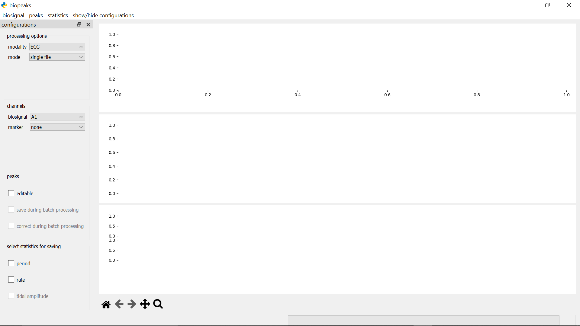
In the menubar, you can find the sections biosignal, peaks, and statistics. These contain methods for the interaction with your biosignals. On the left side, there’s a panel containing configurations that allows you to customize your workflow. You can toggle the visibility of the configurations with show/hide configurations in the menubar. To the right of the configurations is the datadisplay which consists of three panels. The upper panel contains the biosignal as well as peaks identified in the biosignal, while the middle panel can be used to optionally display a marker channel. The lower panel contains any statistics derived from the peaks. Adjust the height of the panels by dragging the segmenters between them up or down. Beneath the datadisplay, in the lower left corner, you find the displaytools. These allow you to interact with the biosignal. Have a look in the functionality section for details on these elements.
Getting started
The following work-flows are meant as an introduction to the interface. Many other
work-flows are possible. Note that biopeaks works with the OpenSignals file format
as well as EDF files, and plain text files (.txt, .csv, .tsv) containing biosignal channels as columns. The functions
used in the exemplary work-flow are described in detail in the functionality section.
extracting ECG features from an OpenSignals file
-
Download the example data (click the
Downloadbutton on the upper right). - Configure the processing options in the configurations:
- Since we want to analyze ECG data, make sure that processing options -> modality is set to “ECG”.
- Set processing options -> mode to “single file”.
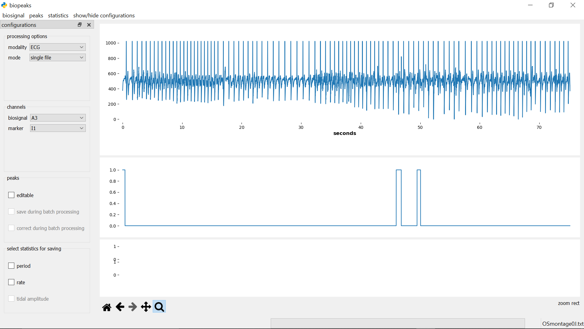
- Set channels -> biosignal to “A3” (ECG has been recorded on analog channel 3) and marker to “I1” (events have been marked in input channel 1).
-
Load the example data using menubar -> biosignal -> load -> Opensignals. More details on loading data can be found here.
-
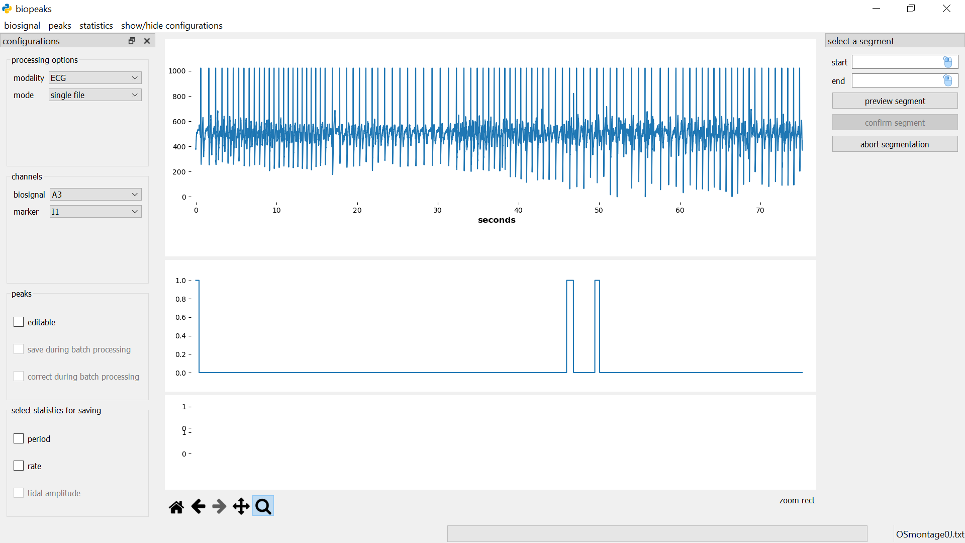
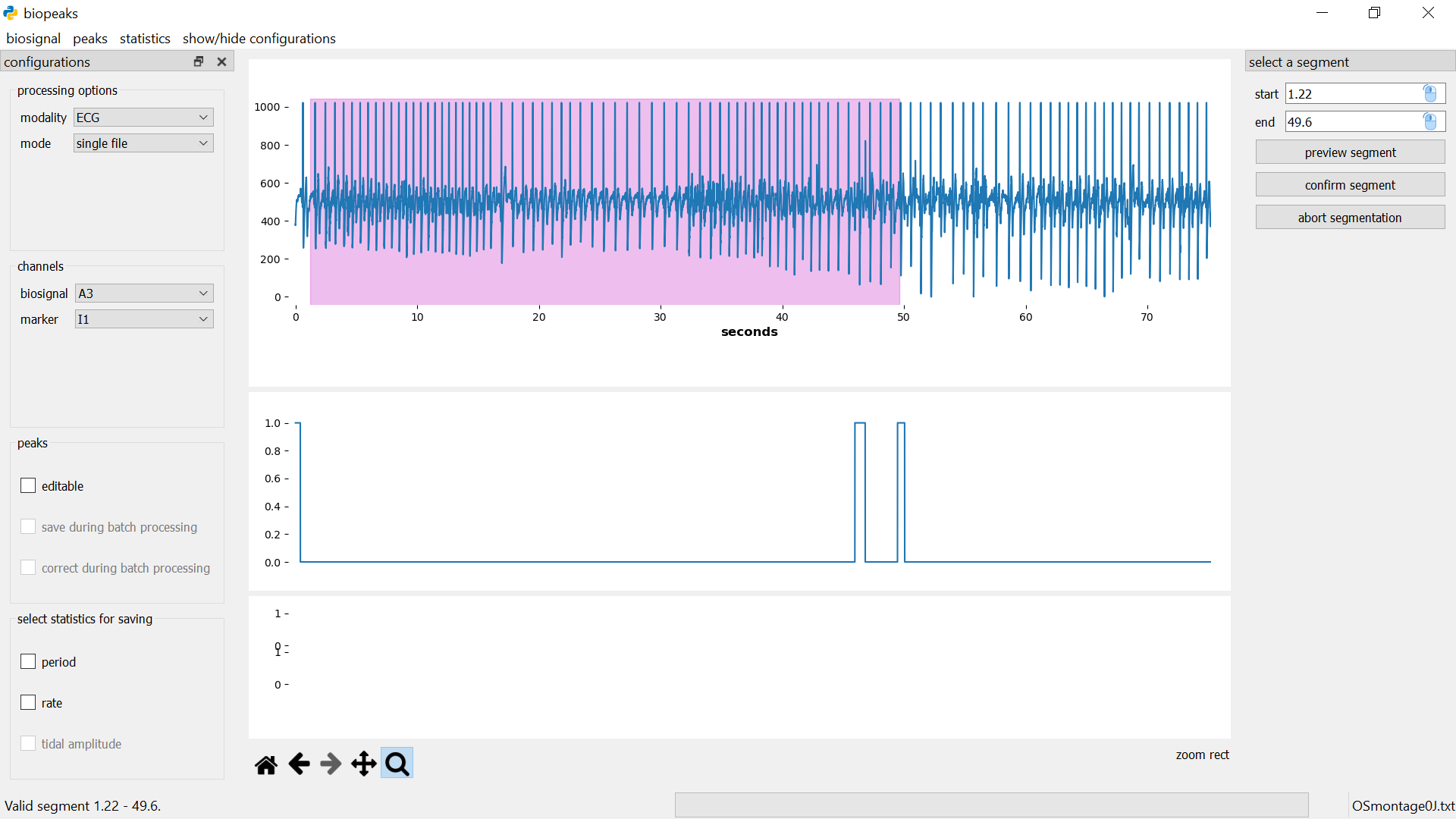
Once the data has been loaded, lets select a segment. menubar -> biosignal -> select segment opens the segmentdialog on the right side of the datadisplay. Select the segment from the second marker at 150 seconds to the end of the signal at 340 seconds by entering “150” and “340” in the
startandendfields respectively. Clickpreview segmentto verify that the correct segment has been selected. Now, clickconfirm segmentto cut out the selection. Note that the original file is not affected by this. More details on segmenting can be found here. -
Now you can identify the R-peaks using menubar -> peaks -> find. Around second 10, you’ll notice irregularities in the placement of the R-peaks. Zoom in on the biosignal by clicking on the magnifying glass in the displaytools. You can now use the mouse cursor to draw a rectangle around the biosignal between seconds 5 and 20. This will result in the magnification of that segment. Note that zooming is easier when you enlarge the panel containing the biosignal by dragging down the gray segmenter underneath the panel. You’ll see a slightly misplaced R-peak around second 11 as well as a missing R-peak at second 13. In the next two steps, we’ll correct these R-peaks using manual and automatic correction. The functionality section contains more details on how to find extrema and use the displaytools.
-
First, lets use autocorrection: menubar -> peaks -> autocorrect. This corrects pronounced irregularities in the R-peaks, such as missing R-peaks or relatively large misplacements. You’ll see that the autocorrection adds the missing R-peak at 13 seconds. However, it does not correct the subtle misplacement of the R-peak at 11 seconds. More details on the autocorrection can be found here.
-
To correct the misplacement at 11 seconds you can use manual peak editing. Check the box next to configurations -> peak -> editable. Now click on the biosignal panel once to enable peak editing. Delete the misplaced R-peak by placing the mouse cursor in it’s vicinity and pressing “d” on your keyboard. Next, you can insert the R-peak at the correct position by placing the mouse cursor on the R-peak at 11 seconds and pressing “a”. You can play around with adding and deleting peaks to get a feeling for how it works. More details on editing peaks can be found here.
-
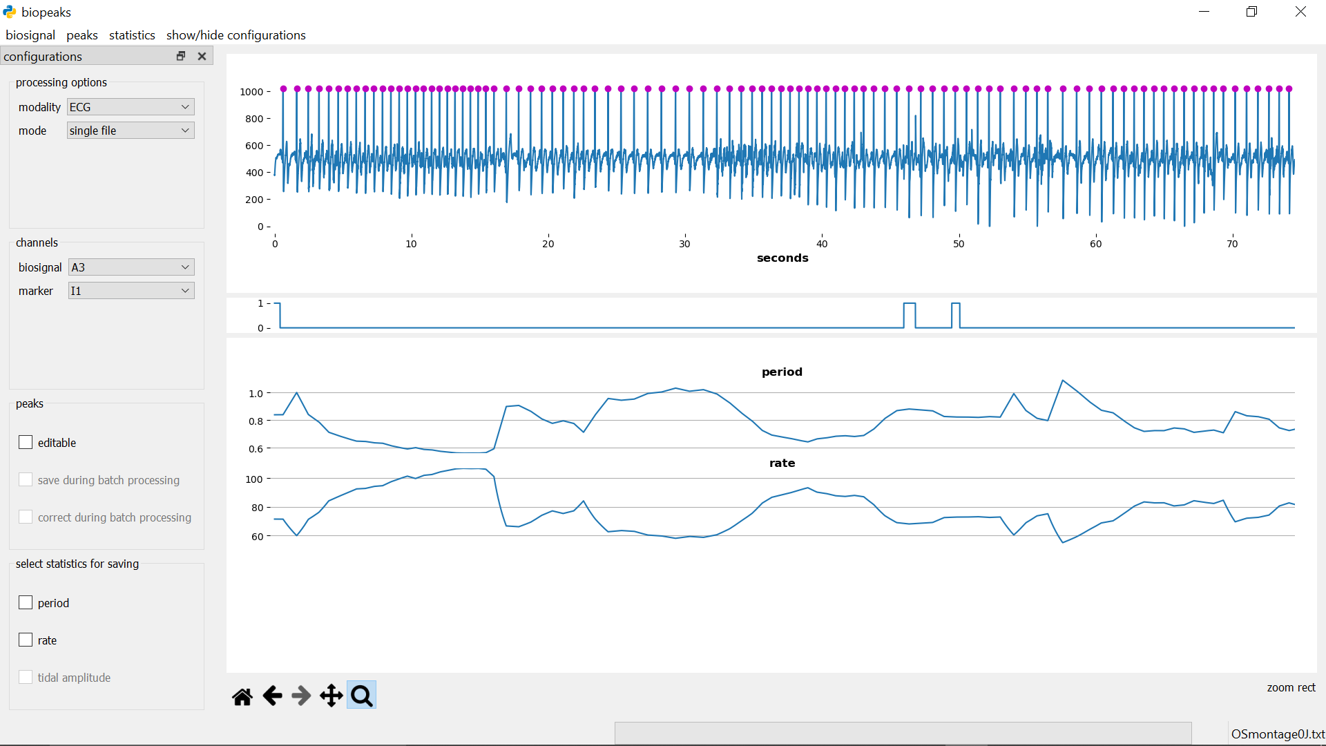
Now you’re ready to extract heart period and heart rate by clicking menubar -> statistics -> calculate. Both statistics will be displayed in the lower panel of the datadisplay. More details on calculating statistics can be found here.
- Finally, to be able to reproduce your results, save the segment (menubar -> biosignal -> save), peaks (menubar -> peaks -> save), and statistics (menubar -> statistics -> save). Prior to saving the statistics, check the boxes next to the statistics that you’d like to save: configurations -> select statictics for saving. You can now use the statistics and/or peaks for further analysis such as averages or heart rate variability.
extracting respiration features from a custom file
You can analyze any plain text file (.txt, .csv, .tsv) as long as it contains biosignal(s) as column(s).
-
Download the example data (click the
Downloadbutton on the upper right). - Configure the processing options in the configurations:
- Since we want to analyze respiration data, make sure that processing options -> modality is set to “RESP”.
- Set processing options -> mode to “single file”.
-
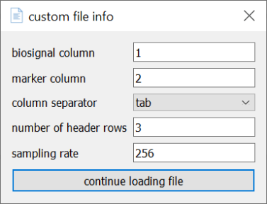
Load the example data using menubar -> biosignal -> load -> Custom. This will pop up a dialog that prompts you for information about the custom file. First, you need to specify which column contains the biosignal. Since the respiration channel is recorded in column 6 of the example data, fill in “6” in the
biosignal columnfield. Similarly, the marker we’d like to display is recorded in column 2. Since the columns of the example data file are separated by tabs, you can select “tab” from thecolumn separatordropdown menu. If the data file contains a header, specify thenumber of header rows. The example data has 3 header rows. Finally, you need to specify thesampling rate. The example data has been recorded at 1000 Hz. Clickcontinue loading fileto select the example data file from your file system. More details on how to load a custom file can be found here. -
Once the biosignal and marker are displayed in the upper and lower datadisplay panels respectively, you can select a segment. menubar -> biosignal -> select segment opens the segmentdialog on the right side of the datadisplay. Select the segment from the start of the recording (0 seconds) to the first marker at 95 seconds by entering “0” and “95” in the
startandendfields respectively. Clickpreview segmentto verify that the correct segment has been selected. Now, clickconfirm segmentto cut out the selection. Note that the original file is not affected by this. More details on segmenting can be found here. -
Now you can use menubar -> peaks -> find to identify the breathing extrema.
-
Once the extrema are displayed on top of the biosignal, you’re ready to extract breathing period, -rate, and -amplitude by clicking menubar -> statistics -> calculate. All three statistics will be displayed in the lower panel of the datadisplay. More details on calculating statistics can be found here.
- Finally, to be able to reproduce your results, save the segment (menubar -> biosignal -> save), breathing extrema (menubar -> peaks -> save), and statistics (menubar -> statistics -> save). Prior to saving the statistics, check the boxes next to the statistics that you’d like to save: configurations -> select statictics for saving. You can now use the statistics and/or peaks for further analysis.
Functionality
- load biosignal
- segment biosignal
- save biosignal
- find peaks
- save peaks
- load peaks
- calculate statistics
- save statistics
- edit peaks
- auto-correct peaks
- batch processing
- displaytools
load biosignal
OpenSignals and EDF
Under configurations -> channels, specify which channel contains the biosignal corresponding to your modality. Optionally, in addition to the biosignal, you can select a marker. This is useful if you recorded a channel that marks interesting events such as the onset of an experimental condition, button presses etc.. You can use the marker to display any other channel alongside your biosignal. Once these options are selected, you can load the biosignal: menubar -> biosignal -> load -> Opensignals or EDF. A dialog will let you select a file.
Plain text files
If you have a .txt, .csv, or .tsv file that contains biosignal channels as columns, you can load a biosignal channel and optionally a marker channel using menubar -> biosignal -> load -> Custom. This will open a dialog that prompts you for some information.
Note that the fields biosignal_column, number of header rows, and sampling rate are required, whereas marker column is optional. In case your file doesn’t have a header, simply put “0” into the number of header rows field. Also make sure to select the correct column separator (“comma” for .csv, “tab” for “tsv”, “colon”, or “space” in case your columns are separated with these characters). Once you’re done, pressing continue loading file opens another dialog that will let you select the file.
Once the biosignal has been loaded successfully it is displayed in the upper datadisplay. If you selected a marker, it will be displayed in the middle datadisplay. The current file name is displayed in the lower right corner of the interface. You can load a new biosignal from either the same file (i.e., another channel) or a different file at any time. Note however that this will remove all data that is currently in the interface.
segment biosignal
menubar -> biosignal -> select segment opens the segmentdialog on the right side of the datadisplay.
Specify the start and end of the segment in seconds either by entering values, or with the mouse. For the latter option, first click on the mouse icon in the respective field and then left-click anywhere on the upper datadisplay to select a time point. To see which time point is currently under the mouse cursor have a look at the x-coordinate displayed in the lower right corner of the datadisplay (displayed when you hover the mouse over the upper datadisplay). If you click preview segment the segment will be displayed as a shaded region in the upper datadisplay but the segment won’t be cut out yet.
You can change the start and end values and preview the segment until you are certain that the desired segment is selected. Then you can cut out the segment with confirm segment. This also closes the segmentdialog. Alternatively, the segmentdialog can be closed any time by clicking abort segmentation. Clicking abort segmentation discards any values that might have been selected. You can segment the biosignal multiple times. Other data (peaks, statistics) will be also be segmented if they are already computed. Note that the selected segment must have a minimum duration of five seconds. Also, after the segmentation, the signal starts at second 0 again. That is, relative timing is not preserved during segmentation. The original file is not affected by the segmentation.
save biosignal
menubar -> biosignal -> save opens a dialog that lets you select a directory and file name for saving the biosignal. Note that saving the biosignal is only possible after segmentation. The file is saved in its original format containing all channels.
find peaks
Before identifying peaks, you need to select the modality of your biosignal
in configurations -> processing options -> modality (“ECG” for
electrocardiogram, “PPG” for photoplethysmogram, and “RESP” for breathing).
This is important since biopeaks uses modality-specific peak detectors.
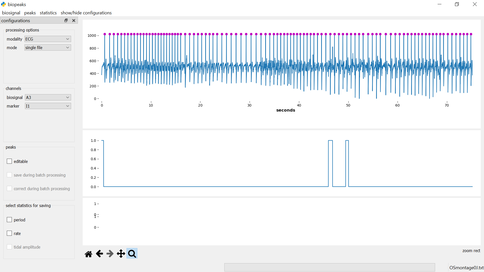
Then, menubar -> peaks -> find automatically identifies the peaks in the
biosignal. The peaks appear as dots displayed on top of the biosignal.
save peaks
menubar -> peaks -> save opens a file dialog that lets you select a
directory and file name for saving the peaks to a CSV file. The format of the
file depends on the modality. For ECG and PPG, biopeaks saves a column containing
the occurrences of R-peaks or systolic peaks respectively in seconds. The first element contains the header
“peaks”. For breathing, biopeaks saves two columns containing the occurrences
of inhalation peaks and exhalation troughs respectively in seconds. The first
row contains the header “peaks, troughs”. Note that if there are less peaks
than troughs or vice versa, the column with less elements will be padded with
a NaN.
load peaks
menubar -> peaks -> load opens a file dialog that lets you select
the file containing the peaks. Note that prior to loading the peaks, you have
to load the associated biosignal. Also, loading peaks won’t work if there are
already peaks in memory (i.e., if there are already peaks displayed in the
upper datadisplay). Note that it’s only possible to load peaks that have
been saved with biopeaks or adhere to the same format. The peaks appear as
dots displayed on top of the biosignal.
calculate statistics
menubar -> statistics -> calculate automatically calculates all possible statistics for the selected modality. The statistics will be displayed in the lowest datadisplay.
save statistics
First select the statistics that you’d like to save: configurations -> select statictics for saving. Then, menubar -> statistics -> save, opens a file dialog that lets you choose a directory and file name for saving a CSV file. The format of the file depends on the modality. Irrespective of the modality the first two columns contain period and rate (if both have been chosen for saving). For breathing, there will be an additional third column containing the tidal amplitude (if it has been chosen for saving). The first row contains the header. Note that the statistics are linearly interpolated to match the biosignal’s timescale (i.e., they represent instantaneous statistics sampled at the biosignal’s sampling rate).
edit peaks
It happens that the automatic peak detection places peaks wrongly or fails to detect some peaks. You can catch these errors by visually inspecting the peak placement. If you spot errors in peak placement you can correct those manually. To do so make sure to select configurations -> peak -> editable. Now click on the upper datadisplay once to enable peak editing. To delete a peak place the mouse cursor in it’s vicinity and press “d”. To add a peak, press “a”. Editing peaks is most convenient if you zoom in on the biosignal region that you want to edit using the displaytools. The statistics in the lowest datadisplay can be a useful guide when editing peaks. Isolated, unusually large or small values in period or rate can indicate misplaced peaks. Note, that when editing breathing extrema, any edits that break the alternation of peaks and troughs (e.g., two consecutive peaks) will automatically be discarded when you save the extrema. If you already calculated statistics, don’t forget to calculate them again after peak editing.
auto-correct peaks
If the modality is ECG or PPG, you can automatically correct the peaks with menubar -> peaks -> autocorrect. Note that the auto-correction tries to spread the peaks evenly across the signal which can lead to peaks that are slightly misplaced. Also, the auto-correction does not guarantee that all errors in peak placement will be caught. It is always good to check for errors manually!
batch processing
There is no substitute for manually checking the biosignal’s quality as well as the placement of the peaks. Manually checking and editing peak placement is the only way to guarantee sensible statistics. Only use batch processing if you are sure that the biosignal’s quality is sufficient!
You can configure the batch processing in the configurations.
To enable batch processing, select
processing options -> mode -> “multiple files”. Make sure to
select the correct modality in the processing options as well. Also select
the desired biosignal channel in channels (for custom files you can
specify the biosignal_column in the file dialog while loading the files). Further, indicate if you’d
like to save the peaks during batch processing: peak options ->
save during batch processing. You can also choose to apply the auto-correction
to the peaks by selecting peak options ->
correct during batch processing. Also, select the statistics you’d like
to save: select statictics for saving. Now, select
all files that should be included in the batch: menubar -> biosignal
-> load. A dialog will let you select the files (select multiple files with
the appropriate keyboard commands of your operating system). Next, a dialog
will ask you to choose a directory for saving the peaks (if you enabled that
option). The peaks will be saved to a file with the same name as the biosignal
file, with a “_peaks.csv” extension.
Finally, a dialog will ask you to select a directory for saving the statistics
(if you chose any statistics for saving). The statistics will be saved to a
file with the same name as the biosignal file, with a “_stats.csv” extension. Once all
dialogs are closed, biopeaks carries out the following actions for each file
in the batch: loading the biosignal, identifying the
peaks, calculating the statistics and finally saving the desired data (peaks
and/or statistics). Note that nothing will be shown in the datadisplay
while the batch is processed. You can keep track of the progress by looking
at the file name displayed in the lower right corner of the interface.
Note that segmentation or peak editing are not possible during batch
processing.
displaytools
The displaytools allow you to interact with the biosignal. Have a look here for a detailed description of how to use them.